Photo by Md Mahdi on Unsplash

1. The goal, and goals

I wondered if you can predict the year‘s world cup with machine learning. Researching a bit further, I came across different approaches, but the stardard solution was a classification model: Classifying the match as

1. Home wins
2. Away wins
3. Draw

For that reason, I figured it would be more interesting to use a different paradigm: Predicting goals scored. With this approach, you can predict expected goals, as well as derive the classification from that. I also decided to use a pretty linear model (combining 2–3 linear with ReLU layers).

To be honest, I definitely did not start this project thinking that this model would yield any real world results. My goal for this project was, and is, to learn data science and machine learning.

2. Getting the data

I used the European Soccer database. It has data over 25k matches, along with detailed team and player attributes. Unfortunately, only 11 european countries are included, which is why my model won‘t be so suitable for predicting games outside of europe. Still, I don‘t want to include other datasets for lack of time needed to restructure the two datasets, and because the combined dataset probably would have severe gaps.

3. Cleaning and parsing the data

This step was completed pretty quickly. Class-attributes, such as low, medium and high had to be switched out for integers, such as 1, 2 and 3. To filter out recurring data, I deleted the class-attributes that were already accompanied by precise numbers (such as 1–100).

Next I made a program that reads all relevant files and combines them into a new one which can be passed directly into the model: The model is trained on a match-basis, where all datapoints are

At first, I just put all remaining datapoints into the model. Data from the match itself, 2 teams and 22 players amounted to 904 parameters in total.

Splitting the dataset into train and test occures in the

4. Training a first model

My first model‘s layer structure combined 3 linear layers with 2 relu layers. Its input features were 904, hidden units 64, and output features 2 (corresponding to the two goal counts for each team).

Furthermore, I used the SGD optimizer with MSE loss.

At first the model had exploding gradients (outputs were nan from the first epoch starting). In response, I lowered it‘s learning rate to ca. 0.0005. With a learning rate this low, I also implemented a scheduler, so that the actual learning rate would not decrease as much with increasing epoch size.

The result? After a slow learning process, the loss decreased from 1.7 to about 1.25.

5. Improving the model

There were a lot of things to improve:

• Firstly, I implemented basic gradient clipping to prevend gradients exploding. This allowed for a higher learning rate. It now is set to 0.005, because a higher one would not yield better results. (Instead, the loss would only jump up and down)
• Secondly, I reduced the number of input features to 504, mainly by filtering out datapoints such as goalkeeper agility, that had a high correlation to other parameters, such as agility, therefore ‘repeating‘ the insight.
• Thirdly, filtering the dataset for matches with too many unknown datapoints reduced the complete dataset to 23k matches. With more dependable values, the model can learn faster.

The last model reached a loss of 1.25 around epoch 600. The new model needed 300 for that. This decreased the loss after about 800 epochs to about 1. Overfitting was not a problem since the loss difference between the test and train set was mostly smaller than 4%.

6. Analyzing predictions

Next up, we should analyze the model. Useful datapoints to consider are:

• Was the winning side predicted correctly? (Winning team or draw was correct)
• Were the goals predicted correctly? (rounded predictions of goals are true)
• Were the predicted goals not far away from the real ones? (rounded predictions of goals are +-1 correct compared to the real goals)

Since the model can’t put out draws, only the goals, the questions remains how to classify those. One solution is to determine the predicted winner first, then see if the difference between both goals is less than, say 5%.

The way we analyze model output is by iterating over the test dataset, making predictions and analyzing them, and then saving them in a csv. Next they an be loaded in a pandas dataframe and plotted. By saving the file, we can use it for further analysis later on.

When comparing the predicted goals vs the real ones, we unfortunately see that there is no real correlation between them. We can see that in following graph. (Actual goals are blue and ascending, their prediction counterparts are red)

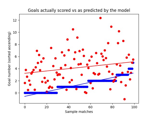
To be exact, this does not mean that the model can’t predict the outcomes. Overall, the prediction accuracy of the match outcome was ca. 42%. However, the model would still loose money when tested in the real world. To be specific, ca 6% per bet.

Analyzing predictions for the test dataset gives us following KPIs:

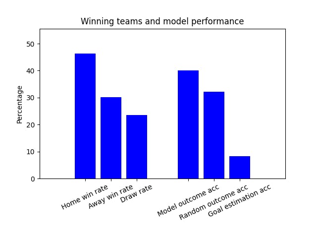
Average gain per bet: - 5.10%
Predictive accuracy (match outcome): 42.19%
Win rates: Home: 46.34% | Away: 30.18% | Draw: 23.48%
More accurate than betting solely on home: - 9.82%
More accurate than betting randomly: 19.96%
Estimation accuracy (goals soft): 7.89%

From this data, we can derive that our model predicts the outcome better than guessing. However, it still was more accurate to always say home wins. This meant that there was still a lot of room for improvement.

8. Lots of monte-carlo simulations

Since betting-odds per match from various providers were also included in the dataset, it‘d be interesting to see how the model would perform against the bookies. Monte-Carlo simulations would be a good fit for this goal.

These were the following variables that we need to consider:

• Number of simulations = 20
• Duration of iterations (number of bets) = 100
• Stake of each bet = 10%
• Starting value (here: starting balance) = 100 (€)

Using the file from analyzing the predictions, we can now shuffle the rows and take a sample list with the length of iterations for each simulation. Each simulation starts with the starting balane. Each iteration, the simulation takes a bet with the current value * stake, and updates the current value with a delta function.

Here is an example:

Simulation 1 has a starting value of 100 and a stake of 0.2 (20%)

1. Iteration 1: The model bets 20 (100 * 0.2) and predicts correctly that the away team wins. Bookies set their odds at 2. This means, that the model wins 20 (20 * (2–1)) and now has a value of 120
2. Iteration 2: The model now bets 24 (120 * 20) and its prediction for this match is wrong. Therefore, it loses the bet value of 24 and has a value of 96.
3. …

These are some of the results:

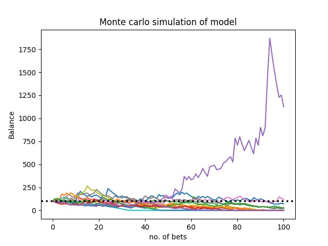
As you can see, it’s just a statistical game: There are always 1–2 outliers that have positive performance, but the far majority spirals down toward 0. This stands in line with the average loss of 6% for each bet the model takes which we calculated earlier.

9. ideas for improvement

My model did not advance beyond a loss of ca 0.95, which probably means that is architecture is not flexible enough to adapt to the dataset enough. This is why newer versions should have more, and deeper layers. Another way to make the model more accurate could be to trim the data set down even further, reducing input complexity.

I consider this project completed for now, but it‘s likely that I will revisit it when I have more expertise and implement new solutions.

Learnings

• More Parameters doesn‘t equal better predictions. It‘s about how these parameters have an effect on the outcome.
• More complex neural networks, like a CNN is likely to be a better option for complex datasets (like this one)
• A dataset has to be prepared thoroughly to avoid errors during training (e.g. through wrong formatting of csv files leading to wrong inputs, which can’t be found easily)
• A custom framework for pytorch is a real time-saver.
• Save models during training to pick the one performing best, so that you don’t have to deal with overfitting (which would increase loss over time)
• For models with lots of input parameters, a low learning rate could be better.

Final Thoughts

Although my model would not do well in a real world situation, I have achieved my main goal: I learned a much about machine learning, and how to visualize data (using matplotlib).

This is where the article ends, but maybe you’ll find an article as interesting on my medium page. Also check out my website, davidewiest.com.

Did you spot anything wrong, or do you have feedback? Please write a comment or note. Thank you!

---

My process of making a soccer game prediction model was originally published in The Modern Scientist on Medium, where people are continuing the conversation by highlighting and responding to this story.